A game's shot chart against the league
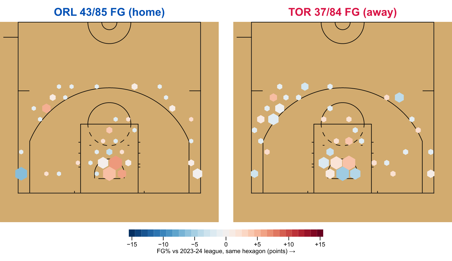
What you'll build: a recap chart for one NBA game. Each team's field-goal
attempts are binned into 2 ft hexagons on a half court. A hexagon's size is how
often the team shot from there, and its colour is how the team's FG% there
compares with the whole league's FG% from the same hexagon over the 2023-24
season. The script also prints the same comparison by zone. Written to
examples/out/shots_vs_league.png.
Needs sportsdataverse ≥ 4.0.0 and @sportsdataverse/* ≥ 0.1.0. Neither is on
npm yet, so build both from source: see the shot chart
tutorial for linking
sdvplot-js.
Sources used
| Source | Host | Call |
|---|---|---|
| ESPN Site API v2 | site.api.espn.com/apis/site/v2/sports/basketball/nba/summary?event=401585607 | sdv.nba.espnNbaSummary({ section: 'plays' | 'header' }) |
| sportsdataverse-data releases | github.com/sportsdataverse/sportsdataverse-data/releases/download/espn_nba_shots/shots_2024.parquet | sdv.nba.loadNbaShots({ seasons: 2024 }) (in the snapshot script) |
@sportsdataverse/sdvplot | (library; no network) | /shots: leagueIndex, cellsVsLeague, sizeCells, diffScale, statsByZone; /plot: surface, shotCells; /export: toPNG; teamColors |
Offline fixtures: test/fixtures/espn/summary_nba.json (Toronto at Orlando,
2024-03-17) and test/fixtures/releases/nba_shots_2024_spots.json (the league
baseline, below). The script also needs @observablehq/plot and jsdom, which
examples/_resolve.mjs takes from the sdvplot-js checkout.
The league baseline
A shot chart needs a league to be compared with. loadNbaShots reads the
espn_nba_shots release: 291,139 rows for 2023-24, every shot in 1,320 games,
including free throws. That is a 3.6 MB download, which a docs build should not
repeat. So tools/snapshots/nba-league-shots.mjs reads it once and keeps the
field-goal attempts counted per ESPN court spot: [x, y, value, attempts, makes].
ESPN records shot locations in whole feet, so this count loses nothing a 1 ft or
coarser binning can see. The 234,063 attempts become 2,310 rows (47 KB), and the
file records the asset's URL, sha256, size and capture time.
Two facts about the release decide how the snapshot is made, and both were checked against the data, not assumed:
- The release covers this game. It holds all 169 field-goal attempts of
game 401585607, at the same spots as the summary capture
(
coordinate_x_raw/coordinate_y_raware the summary'scoordinate_x/coordinate_y). So the baseline includes the game, as 169 of 234,063 attempts. - A miss has no point value. The release's
score_valueis the points a shot scored, so it is 0 on every miss, and the shot kit needs a 2 or a 3 for every attempt. The snapshot labels a miss by its spot: a three is 21.5 ft or more to the side of the hoop and at most 9 ft up the floor (a corner three), or 23.25 ft or more away. Those are the 22 ft and 23.75 ft lines, read short because ESPN rounds down to whole feet. The rule agrees with the scorer on 99.95% of the season's 110,857 makes and on all 169 attempts of this game, where ESPN'spointsAttemptedgives the answer.
test/tutorial-fixtures.test.js checks the snapshot against the summary capture
on every run. With SDV_LIVE=1 it downloads the asset again, checks the sha256
and re-derives every row.
From ESPN's frame to the shot kit's
@sportsdataverse/sdvplot/shots works in the stats.nba.com "legacy" frame:
tenths of a foot, with the hoop at the origin and y running toward half court.
ESPN's frame was measured in the play-by-play tutorial: x is
feet across the court with the hoop at 25, and y is feet toward half court with
the hoop at 1. One shift and one scale join them:
x_legacy = (coordinate_x − 25) × 10
y_legacy = (coordinate_y −  1) × 10
Each shot becomes a ShotRow: those two coordinates, shot_distance in whole
feet, shot_value (ESPN's points_attempted for the game, the snapshot's
value for the league) and shot_result. The script maps the game and the
league through the same function, so a mirror image between the two frames
would move both alike. The printed table still merges the left and right corner
threes, because nothing here shows which side of ESPN's frame is the left
corner.
Before grouping plays by team, the script checks that the header's team ids and
the plays' team_id have the same type. Both are strings, as every sdv-js id
is.
Hexagons against the league
leagueIndex(league, { radius: 20 }) bins every league attempt into 2 ft
hexagons and keeps each one's attempts and FG%, along with the league's rate
for each of the six zones. cellsVsLeague(teamShots, index) bins a team's
attempts on the same lattice, so each team hexagon has a league hexagon with
the same centre, and attaches that league FG% to it. (A hexagon the league shot
from fewer than 25 times uses its zone's rate.) sizeCells sizes the hexagons
by attempts, and shotCells colours each one with diffScale by its FG% minus
the league's. That difference is shrunk: 25 league-rate attempts are added
before it is taken. A hexagon a team made 3 of 3 from, where the league shot 40%,
shows +6 points, not +60. For a single game this is what you want: one
hot hand in one hexagon should not read as a trend. It also means one game's
colours stay pale. The zone table, which has more attempts per row, carries the
sharper comparison.
The chart is drawn by Observable Plot in Node: Plot.plot({ document }) with a
jsdom document. toPNG (resvg) then rasterises the two courts and the key,
set side by side in one SVG. Plot's own colour legend paints a <canvas>,
which jsdom lacks, so the key is a strip of Plot.rect marks in the scale's
colours.
The script
// 94 — A game's shot chart against the league: ESPN plays + the 2023-24 league
// baseline → sdvplot hexagons coloured by FG% vs the league → PNG.
//
// Shows: ESPN summary `plays` for one game, mapped into the shot kit's frame
// (@sportsdataverse/sdvplot/shots: legacy tenths of a foot, hoop at the origin);
// `leagueIndex` over every 2023-24 field-goal attempt (the `espn_nba_shots`
// release, counted per ESPN spot in a committed snapshot); `cellsVsLeague` +
// `sizeCells` per team; `surface` + `shotCells` drawn with Observable Plot in
// Node (jsdom), then rasterised by `toPNG` (resvg). Writes
// examples/out/shots_vs_league.png. sdvplot-js is UNPUBLISHED (see README.md).
//
// Frame (fitted in 02_nba_pbp_shots.mjs, MAE 0.3 ft): ESPN `coordinate_x` is feet
// across the court with the hoop at 25, `coordinate_y` feet toward half court with
// the hoop at 1, whole feet, one basket for both teams. So
//   x_legacy = (coordinate_x - 25) * 10,  y_legacy = (coordinate_y - 1) * 10.
// Free throws carry a sentinel and are dropped. `shot_value` is ESPN's
// `points_attempted` (2 or 3); the shot kit reads it for the zones.
//
// The league snapshot: test/fixtures/releases/nba_shots_2024_spots.json, written by
// tools/snapshots/nba-league-shots.mjs from `sdv.nba.loadNbaShots({ seasons: 2024 })`
// (provenance inside the file). It includes this game: the release carries all
// 169 of its field-goal attempts, at the same spots as the summary below.
//
// Sources: ESPN Site API v2 — site.api.espn.com/apis/site/v2/sports/basketball/nba/summary?event=401585607
// and the sportsdataverse-data release espn_nba_shots/shots_2024.parquet.
// Offline fixtures: test/fixtures/espn/summary_nba.json (ORL vs TOR, 2024-03-17) + the snapshot above.

import { mkdirSync, readFileSync, writeFileSync } from 'node:fs';
import * as Plot from '@observablehq/plot';
import { JSDOM } from 'jsdom';
import sdv from 'sportsdataverse';
import { teamColors } from '@sportsdataverse/sdvplot';
import { toPNG } from '@sportsdataverse/sdvplot/export';
import { shotCells, surface } from '@sportsdataverse/sdvplot/plot';
import { cellsVsLeague, diffScale, leagueIndex, sizeCells, statsByZone } from '@sportsdataverse/sdvplot/shots';
import { setup } from './_offline.mjs';
import { printTable, round } from './_util.mjs';

setup();

const EVENT_ID = 401585607;
const FONT = 'Arial, Helvetica, sans-serif'; // resvg draws text with the system's fonts; Plot's default system-ui resolves oddly there
const HEX = { radius: 20 }; // 2 ft hexagons: one game is ~85 attempts a team, so coarser than a season chart's 1.5 ft

/** One ESPN shot → the shot kit's ShotRow (legacy tenths, hoop at the origin). */
const shotRow = (x, y, value, made) => {
  const dx = x - 25;
  const dy = y - 1;
  return { x_legacy: dx * 10, y_legacy: dy * 10, shot_distance: Math.round(Math.hypot(dx, dy)), shot_value: value, shot_result: made ? 'Made' : 'Missed' };
};

// --- the game ------------------------------------------------------------------
const header = await sdv.nba.espnNbaSummary({ event_id: EVENT_ID, parsed: true, section: 'header' });
const competitors = JSON.parse(header[0].competitions)[0].competitors;
const teams = competitors.map((c) => ({ id: c.team.id, abbr: c.team.abbreviation, homeAway: c.homeAway, score: c.score }));

const plays = await sdv.nba.espnNbaSummary({ event_id: EVENT_ID, parsed: true, section: 'plays' });
const attempts = plays.filter((p) => p.shooting_play && p.coordinate_x > -100 && !/free throw/i.test(p.text));
// The join key: header team ids and play team ids must be the same type before we group on them.
const idTypes = new Set([...teams.map((t) => typeof t.id), ...attempts.map((p) => typeof p.team_id)]);
if (idTypes.size !== 1) throw new Error(`team_id types disagree between header and plays: ${[...idTypes]}`);

// --- the league ------------------------------------------------------------------
const snapshot = JSON.parse(readFileSync(new URL('../test/fixtures/releases/nba_shots_2024_spots.json', import.meta.url), 'utf8'));
const league = snapshot.spots.flatMap(([x, y, value, n, makes]) =>
  Array.from({ length: n }, (_, i) => shotRow(x, y, value, i < makes))
);
const index = leagueIndex(league, HEX);
const leagueZones = statsByZone(league);

// --- per team: cells vs league, zones vs league ---------------------------------------
const doc = new JSDOM('').window.document;
const court = surface('nba', { displayRange: 'defense', rotation: 90 });
const scale = diffScale();
const colors = await teamColors('nba', teams.map((t) => t.id), { which: 'primary' });
const zoneRows = [];
const panels = [];
const titles = [];
for (const [i, team] of teams.entries()) {
  const shots = attempts.filter((p) => p.team_id === team.id).map((p) => shotRow(p.coordinate_x, p.coordinate_y, p.points_attempted, p.scoring_play));
  const cells = cellsVsLeague(shots, index);
  const zones = statsByZone(shots);
  // corners merged: ESPN's left/right handedness against the legacy frame is not verified
  const merge = (z) => ({
    restricted_area: z.restricted_area,
    paint: z.paint,
    mid_range: z.mid_range,
    corner_3: { attempts: z.corner_3_left.attempts + z.corner_3_right.attempts, makes: z.corner_3_left.makes + z.corner_3_right.makes },
    above_break_3: z.above_break_3,
  });
  const lz = merge(leagueZones);
  for (const [zone, s] of Object.entries(merge(zones))) {
    const fg = s.attempts ? s.makes / s.attempts : null;
    const lfg = lz[zone].makes / lz[zone].attempts;
    zoneRows.push({ team: team.abbr, zone, fga: s.attempts, fgm: s.makes, fg_pct: round(fg, 3), league_fg_pct: round(lfg, 3), diff_pts: fg == null ? null : round((fg - lfg) * 100, 1) });
  }
  const fga = shots.length;
  const fgm = shots.filter((s) => s.shot_result === 'Made').length;
  titles.push({ text: `${team.abbr} ${fgm}/${fga} FG (${team.homeAway})`, color: colors[i] });
  panels.push(
    Plot.plot({
      ...court.scales,
      document: doc,
      style: { fontFamily: FONT },
      width: 360,
      marks: [
        ...court.marks,
        shotCells(cells, { r: sizeCells(cells, HEX).r, frame: 'nba-legacy-vertical', scale }),
      ],
    })
  );
}

// --- one PNG: the two courts side by side, a legend underneath ------------------------
const pts = (d) => (d === 0 ? '0' : `${d > 0 ? '+' : '−'}${Math.abs(d * 100).toFixed(0)}`);
// Plot.legend's continuous ramp paints a <canvas>, which jsdom lacks: draw the key as rects in the scale's colours.
const steps = Array.from({ length: 31 }, (_, i) => round(-0.15 + i * 0.01, 2));
const legend = Plot.plot({
  document: doc,
  style: { fontFamily: FONT },
  width: 360,
  height: 46,
  marginTop: 4,
  marginBottom: 30,
  x: { domain: [-0.155, 0.155], ticks: [-0.15, -0.1, -0.05, 0, 0.05, 0.1, 0.15], tickFormat: pts, label: 'FG% vs 2023-24 league, same hexagon (points) →', labelAnchor: 'center' },
  y: { axis: null },
  color: { type: 'identity' },
  marks: [Plot.rect(steps, { x1: (d) => d - 0.005, x2: (d) => d + 0.005, y1: 0, y2: 1, fill: (d) => scale(d) })],
});
const w = panels.map((p) => Number(p.getAttribute('width')));
const h = Math.max(...panels.map((p) => Number(p.getAttribute('height'))));
const W = w[0] + w[1] + 24;
const TOP = 36; // a title band above the courts
const H = TOP + h + 64;
const nested = (svg, x, y) => {
  svg.setAttribute('x', String(x));
  svg.setAttribute('y', String(y));
  return svg.outerHTML;
};
const svg =
  `<svg xmlns="http://www.w3.org/2000/svg" width="${W}" height="${H}" viewBox="0 0 ${W} ${H}" font-family="${FONT}">` +
  `<rect width="${W}" height="${H}" fill="white"/>` +
  titles.map((t, i) => `<text x="${i === 0 ? w[0] / 2 : w[0] + 24 + w[1] / 2}" y="26" text-anchor="middle" font-size="18" font-weight="bold" fill="${t.color}">${t.text}</text>`).join('') +
  nested(panels[0], 0, TOP) +
  nested(panels[1], w[0] + 24, TOP) +
  nested(legend, (W - 360) / 2, TOP + h + 8) +
  '</svg>';
mkdirSync(new URL('./out/', import.meta.url), { recursive: true });
writeFileSync(new URL('./out/shots_vs_league.png', import.meta.url), await toPNG(svg, { scale: 2 }));

printTable(
  teams.map((t, i) => ({ team: t.abbr, team_id: t.id, home_away: t.homeAway, score: t.score, color: colors[i] })),
  ['team', 'team_id', 'home_away', 'score', 'color'],
  2,
  `Game ${EVENT_ID} vs a league of ${snapshot.provenance.field_goal_attempts} attempts (${snapshot.provenance.games} games)`
);
printTable(zoneRows, ['team', 'zone', 'fga', 'fgm', 'fg_pct', 'league_fg_pct', 'diff_pts'], 10, 'FG% by zone against the league → examples/out/shots_vs_league.png');
This script imports the unpublished @sportsdataverse/* packages, and toPNG
needs the native @resvg/resvg-js, which a WebContainer cannot load. Build
sdvplot-js locally and run it from examples/.
Output
Output of node examples/94_sdvplot_shots_vs_league.mjs (offline, against the committed fixtures):
## Game 401585607 vs a league of 234063 attempts (1320 games)
| team | team_id | home_away | score | color   |
| ---- | ------- | --------- | ----- | ------- |
| ORL  | 19      | home      | 111   | #0150b5 |
| TOR  | 28      | away      | 96    | #d91244 |
(2 rows, all shown)

## FG% by zone against the league → examples/out/shots_vs_league.png
| team | zone            | fga | fgm | fg_pct | league_fg_pct | diff_pts |
| ---- | --------------- | --- | --- | ------ | ------------- | -------- |
| ORL  | restricted_area | 29  | 23  | 0.793  | 0.653         | 14       |
| ORL  | paint           | 16  | 7   | 0.438  | 0.439         | -0.2     |
| ORL  | mid_range       | 4   | 2   | 0.5    | 0.419         | 8.1      |
| ORL  | corner_3        | 16  | 4   | 0.25   | 0.388         | -13.8    |
| ORL  | above_break_3   | 20  | 7   | 0.35   | 0.357         | -0.7     |
| TOR  | restricted_area | 33  | 20  | 0.606  | 0.653         | -4.7     |
| TOR  | paint           | 12  | 4   | 0.333  | 0.439         | -10.6    |
| TOR  | mid_range       | 8   | 5   | 0.625  | 0.419         | 20.6     |
| TOR  | corner_3        | 5   | 1   | 0.2    | 0.388         | -18.8    |
| TOR  | above_break_3   | 26  | 7   | 0.269  | 0.357         | -8.8     |
(10 rows, all shown)
What it shows
Orlando won 111-96. The Magic made 23 of 29 in the restricted area, 14 points above the league's 65.3%; on the chart those are the large reddish hexagons under the basket. Toronto shot more at the rim (33 attempts) and made 20, 4.7 points below the league.
Both teams were cold from three. Orlando went 4 of 16 from the corners, and the big blue hexagon in one corner is most of that. Toronto took 26 above-the-break threes and made 7, 8.8 points below the league's 35.7%. Toronto's best zone was the mid-range, 5 of 8. That is +20.6 points on paper, but it is only eight shots, which is why the shrunk mid-range hexagons barely colour.
The totals match ESPN's box score (Orlando 43-85 with 11-36 from three, Toronto 37-84 with 8-31), which checks the zone split and the three-point labels together.
Variations
- Another game: change
EVENT_IDto any 2023-24 game. The snapshot already holds the league, andSDV_LIVE=1fetches the summary. - Another season: run
tools/snapshots/nba-league-shots.mjswithSEASONchanged, then point the script at the new file. - Square cells:
{ shape: 'square', side: 20 }in place of{ radius: 20 }, andshotCells(cells, { shape: 'square', … }). diffScale({ theme: 'dark' })for a dark page, orprior: 0inshotCellsfor the unshrunk difference.
Work through it live
- sdvplot-js shot charts guide,
with the same
cellsVsLeague/shotCellspipeline on a full season of Brooklyn shots, and its shot dashboard example. - Rendering in Node (jsdom,
linkedom,
toSVG) and exporting PNGs. - The sdvplot-js notebooks, in particular surfaces.
Next steps
- Shot chart with sdvplot + sporty: the raw shots, one dot each, on a sporty court.
- NFL standings as a publication table: sdvtables to PNG.