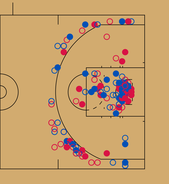
A shot chart: ESPN plays on a sporty court, coloured by sdvplot
What you'll build: an SVG shot chart for one NBA game — the sporty NBA half court with one circle per field-goal attempt, filled when made, in each team's primary colour from sdvplot — plus the table of mapped coordinates that feeds it.
Sources used
| Source | Host | Call |
|---|---|---|
| ESPN Site API v2 | site.api.espn.com/apis/site/v2/sports/basketball/nba/summary?event=401585607 | sdv.nba.espnNbaSummary({ section: 'plays' | 'header' }) |
@sportsdataverse/sporty | (library, no network) | basketballCourt('nba', { displayRange: 'offense' }), toSurfaceFrame, toSVG |
@sportsdataverse/sdvplot | (library; bundled team index, no network) | teamColors('nba', ids, { which: 'primary' }) |
Offline fixture: test/fixtures/espn/summary_nba.json (Toronto at Orlando,
2024-03-17).
sdvplot-js is not published yet
@sportsdataverse/sdvplot (team identity: colours, logos, headshots — the
TypeScript port of sdvplot / sdvplotR) and @sportsdataverse/sporty (sport
surfaces — the port of sportyR / sportypy) live in
sportsdataverse/sdvplot-js and
are not on npm. The repo's examples/package.json links them from a
sibling checkout with file: paths; to run this tutorial:
git clone https://github.com/sportsdataverse/sdvplot-js <two dirs above this repo>/sdvplot-js
cd sdvplot-js && pnpm install
(cd packages/sporty && npx tsup) && (cd packages/sdvplot && npx tsup)
cd <this repo>/examples && npm install    # resolves the file: links
node 90_sdvplot_shot_chart.mjs            # writes examples/out/shot_chart.svg
examples/README.md has the details (and what to do if your checkout lives
elsewhere). Both packages are ESM-only, Node ≥ 20.18.1, no runtime
dependencies; sdvplot's team index is bundled, so colours resolve offline.
The coordinate mapping, fitted
ESPN's shot frame was established empirically in the
play-by-play tutorial by fitting the hoop against the
"N-foot" distances ESPN writes into each play (four games, one committed and
asserted by test/examples-shot-frame.test.js, MAE 0.3 ft):
coordinate_x is feet across the court (0–50, hoop at 25), coordinate_y is
feet from the hoop toward half court (hoop at y = 1), both teams are
normalised onto one basket in every period, and free throws carry a
−214748340 / −214748365 sentinel.
sporty's NBA court is centre-origin feet: x runs along the length (−47 to
47), y across (−25 to 25), and displayRange: 'offense' shows the x ≥ 0
half with the hoop at x = 41.75 (47 − 5.25). The two frames line up with one
affine map:
surface_x = 41.75 − coordinate_y
surface_y = coordinate_x − 25
sporty ships named frames for stats.nba.com (nba-legacy: tenths of a foot,
hoop origin, pair with displayRange: 'defense'), HockeyTech's two canvases,
and ESPN football's 0–100 yardline — but none for ESPN basketball, so the
script passes the mapping as a Frame object ({ x: (row) => …, y: (row) => … })
to toSurfaceFrame, which appends surface_x / surface_y to each row
(and returns null for the free-throw sentinel). The rendered chart is the
check: dunks and layups cluster at the hoop, threes sit just outside the arc,
corner threes land in the corners. If ESPN ever changes the frame, the
distance table in the play-by-play tutorial moves first.
Rendering
toSVG(scene, { width }) draws the court as a viewBox in feet with the
y-axis flipped inside a <g transform="scale(1,-1)">. There is no overlay
helper yet, so the script inserts its <circle> elements into that same group
before </g></svg> — anything placed there uses surface coordinates directly,
no scaling needed. teamColors('nba', ['19', '28'], { which: 'primary' })
resolves the ESPN team ids straight from the summary header (sdvplot's nba
canonical team_id is the ESPN id) to #0150b5 (Orlando) and #d91244
(Toronto).
The script
// 90 — Shot chart: ESPN NBA plays → a sporty court → SVG with sdvplot team colours.
//
// Shows: ESPN summary `plays` (coordinate_x / coordinate_y) mapped onto a
// @sportsdataverse/sporty NBA half court and rendered with `toSVG`, with each
// team's shots coloured by @sportsdataverse/sdvplot `teamColors`. Written to
// examples/out/shot_chart.svg. Both packages are UNPUBLISHED (see README.md).
//
// Coordinate mapping (fitted, not assumed — see 02_nba_pbp_shots.mjs and
// test/examples-shot-frame.test.js): fitting the hoop against the "N-foot"
// distance in each play's text on four ESPN basketball captures (one committed)
// gives hoop = (25, 1) with MAE 0.3 ft, so ESPN's frame is
//   x: feet across the court, 0..50, hoop at 25
//   y: feet from the hoop toward half court, -1..~31 (hoop at y = 1)
//   both teams on ONE basket in every period (no side flip)
//   free throws = sentinel (-214748340, -214748365) → dropped
// sporty's NBA court is centre-origin feet: x along the length (-47..47), y across
// (-25..25); `displayRange: "offense"` shows x in 0..47 with the hoop at x = 41.75
// (47 - 5.25). So:  surface_x = 41.75 - (coordinate_y - 1),  surface_y = coordinate_x - 25.
// sporty has no built-in ESPN basketball frame (its `nba-legacy` frame is for
// stats.nba.com LOC_X/LOC_Y, tenths of a foot); we pass the mapping as `from`.
//
// Sources: ESPN Site API v2 — site.api.espn.com/apis/site/v2/sports/basketball/nba/summary?event=401585607
// Offline fixture: test/fixtures/espn/summary_nba.json (ORL vs TOR, 2024-03-17).

import { mkdirSync, writeFileSync } from 'node:fs';
import sdv from 'sportsdataverse';
import { basketballCourt, toSurfaceFrame } from '@sportsdataverse/sporty';
import { toSVG } from '@sportsdataverse/sporty/svg';
import { teamColors } from '@sportsdataverse/sdvplot';
import { setup } from './_offline.mjs';
import { printTable, round } from './_util.mjs';

setup();

const EVENT_ID = 401585607;
const ESPN_NBA_FRAME = {
  x: (r) => (r.y == null || r.y < -100 ? null : 41.75 - (r.y - 1)),
  y: (r) => (r.x == null || r.x < -100 ? null : r.x - 25),
  description: 'ESPN basketball plays: x across (0-50, hoop 25), y from the hoop toward half court → sporty offense half',
};

const header = await sdv.nba.espnNbaSummary({ event_id: EVENT_ID, parsed: true, section: 'header' });
const competitors = JSON.parse(header[0].competitions)[0].competitors;
const teams = Object.fromEntries(competitors.map((c) => [c.team.id, c.team.abbreviation]));
const teamIds = Object.keys(teams);

const plays = await sdv.nba.espnNbaSummary({ event_id: EVENT_ID, parsed: true, section: 'plays' });
const shots = toSurfaceFrame(
  plays.filter((p) => p.shooting_play && p.coordinate_x > -100 && !/free throw/i.test(p.text)),
  { from: ESPN_NBA_FRAME, x: 'coordinate_x', y: 'coordinate_y' }
);

// Team colours resolve from sdvplot's bundled index (ESPN team ids work directly; no network).
const colors = await teamColors('nba', teamIds, { which: 'primary' });
const colorOf = Object.fromEntries(teamIds.map((id, i) => [id, colors[i]]));

printTable(
  shots.map((s) => ({ team: teams[s.team_id], made: s.scoring_play, x_espn: s.coordinate_x, y_espn: s.coordinate_y, surface_x: round(s.surface_x, 2), surface_y: s.surface_y, text: s.text })),
  ['team', 'made', 'x_espn', 'y_espn', 'surface_x', 'surface_y', 'text'],
  6,
  'Shots mapped onto the sporty court'
);

// Render: court SVG + one <circle> per shot inside the same y-flipped group.
const court = basketballCourt('nba', { displayRange: 'offense' });
const svg = toSVG(court, { width: 720 });
const marks = shots
  .map((s) => `<circle cx="${s.surface_x.toFixed(2)}" cy="${s.surface_y.toFixed(2)}" r="0.9" fill="${s.scoring_play ? colorOf[s.team_id] : 'none'}" stroke="${colorOf[s.team_id]}" stroke-width="0.25"/>`)
  .join('');
const out = svg.replace('</g></svg>', `${marks}</g></svg>`);

mkdirSync(new URL('./out/', import.meta.url), { recursive: true });
writeFileSync(new URL('./out/shot_chart.svg', import.meta.url), out);

printTable(
  teamIds.map((id) => ({ team: teams[id], color: colorOf[id], fga: shots.filter((s) => s.team_id === id).length, fgm: shots.filter((s) => s.team_id === id && s.scoring_play).length })),
  ['team', 'color', 'fga', 'fgm'],
  2,
  'Legend (filled = made, hollow = missed) → examples/out/shot_chart.svg'
);
This script imports @sportsdataverse/sdvplot / @sportsdataverse/sporty, which are not published to npm yet, so a sandbox cannot install them. Build sdvplot-js locally as described above and run it from examples/.
Output
Output of node examples/90_sdvplot_shot_chart.mjs (offline, against the committed fixtures):
## Shots mapped onto the sporty court
| team | made  | x_espn | y_espn | surface_x | surface_y | text                       |
| ---- | ----- | ------ | ------ | --------- | --------- | -------------------------- |
| ORL  | true  | 25     | 3      | 39.75     | 0         | Franz Wagner makes drivin… |
| TOR  | true  | 26     | 2      | 40.75     | 1         | Kelly Olynyk makes drivin… |
| ORL  | false | 2      | 2      | 40.75     | -23       | Gary Harris misses 23-foo… |
| ORL  | true  | 27     | 2      | 40.75     | 2         | Paolo Banchero makes 2-fo… |
| TOR  | false | 23     | 3      | 39.75     | -2        | Gary Trent Jr. misses dri… |
| TOR  | false | 24     | 2      | 40.75     | -1        | Kelly Olynyk misses two p… |
(169 rows, first 6 shown)

## Legend (filled = made, hollow = missed) → examples/out/shot_chart.svg
| team | color   | fga | fgm |
| ---- | ------- | --- | --- |
| ORL  | #0150b5 | 85  | 43  |
| TOR  | #d91244 | 84  | 37  |
(2 rows, all shown)
Variations
- The stats.nba.com
shotchartdetailendpoint (sdv.nba.nba_stats_shotchartdetail, impersonating transport required) carriesLOC_X/LOC_Yin sporty'snba-legacyframe:toSurfaceFrame(rows, { from: 'nba-legacy', x: 'loc_x', y: 'loc_y' })withdisplayRange: 'defense'. basketballCourt('wnba', …)/('ncaa', …)for the other leagues; the ESPN frame is the same (the WNBA capture fitted the same hoop).hockeyRink('nhl')+ thedetails_x_coord/details_y_coordfrom the NHL tutorial is the hockey equivalent (NHL coordinates are already centre-origin feet).
Next steps
- Standings bars in team colours —
paletteandlogoUrl. - Roster table with headshots —
headshotUrl.